Δ.72 — NASA C-MAPSS Turbofan Degradation

Key Results

100%

Δ Detection Rate

93%

Variance Detection Rate

185

Mean Δ Lead (cycles)

83

Mean Var Lead (cycles)

109

Δ Advantage (cycles)

89%

Life Remaining at Alert

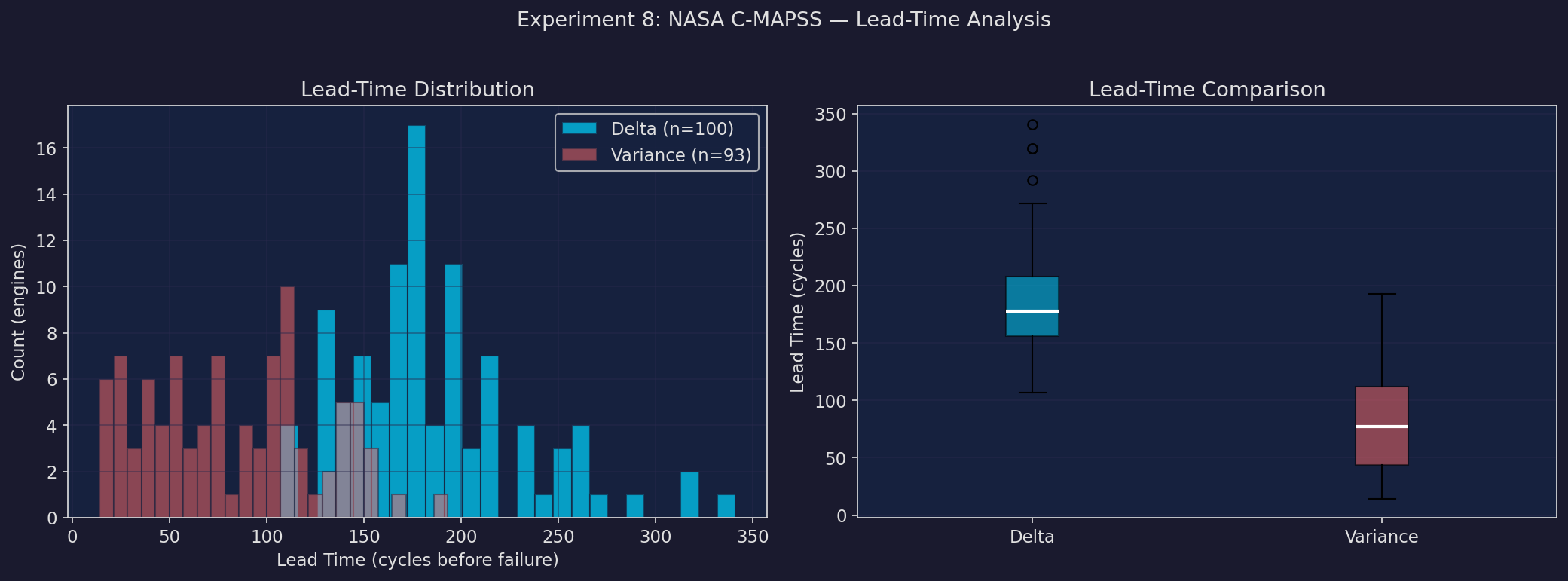
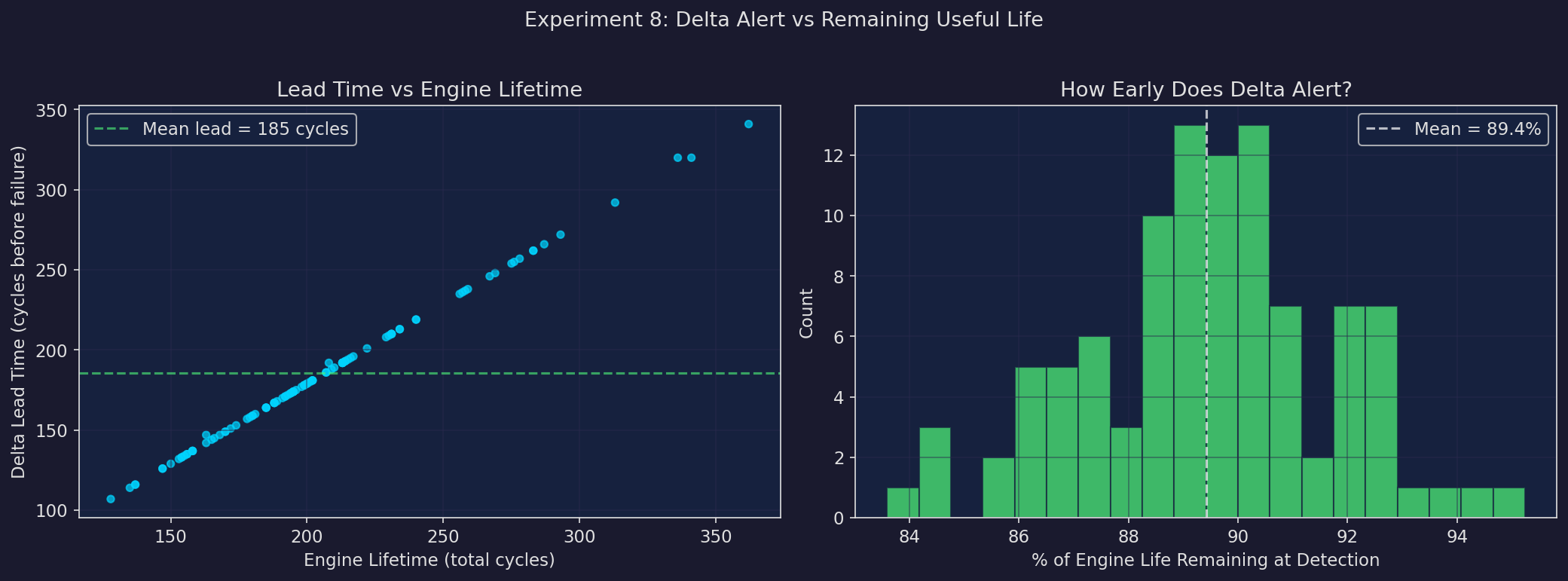
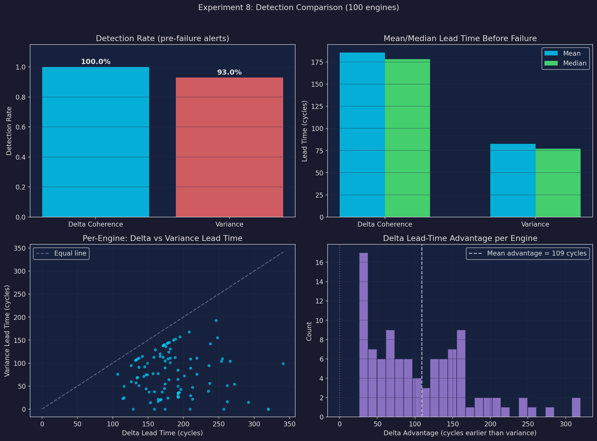
Across 100 NASA C-MAPSS turbofan engines, the Δ coherence metric achieved 100% detection rate with a mean lead time of 185 cycles before failure. Variance-based detection caught 93% of failures with only 83 cycles mean lead. On average, Δ alerts 109 cycles earlier than variance — with 89% of engine life still remaining at first alert.

Method Comparison

Δ Coherence

Detection rate: 100%

Mean lead: 185 cycles

Median lead: 178 cycles

Missed: 0 engines

Variance

Detection rate: 93%

Mean lead: 83 cycles

Median lead: 77 cycles

Missed: 7 engines

Experiment Plots

Plot 01

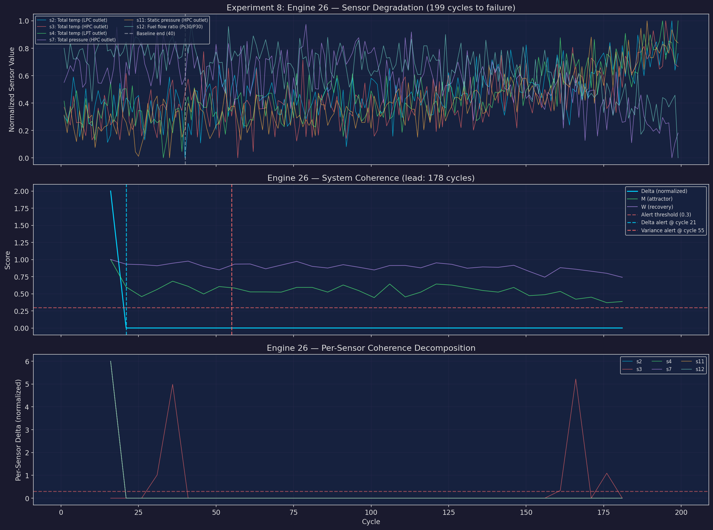
Example Engine Degradation — Engine #26

Top: 6 sensor traces (normalized) showing progressive degradation. Middle: system-level Δ coherence, M (attractor memory), and W (recovery) with alert thresholds. Bottom: per-sensor Δ decomposition.

Example engine degradation with coherence overlay

Sensor degradation becomes visible in raw traces only in the final ~30% of life. Δ coherence detects the structural departure from baseline within the first few windows after the healthy period. Early Detection

Plot 02

Lead-Time Distribution

How many cycles before failure does each method alert? Distribution across all 100 engines.

Δ lead times span 107 to 341 cycles with a tight distribution. Variance lead times are shorter and more dispersed, with 7 engines receiving no warning at all. Consistent

Plot 03

Δ Alert vs Remaining Useful Life

Left: lead time vs engine total lifetime. Right: what percentage of engine life remains when Δ first alerts?

Δ consistently alerts with 89% of engine life remaining, regardless of total engine lifetime. This means the framework scales naturally — longer-lived engines get proportionally more warning. Scalable

Plot 04

Detection Comparison: Δ vs Variance

Detection rates, lead times, per-engine scatter, and advantage distribution.

Every single engine where Δ detected failure, it did so earlier than variance. The mean advantage of 109 cycles represents significant actionable lead time for maintenance scheduling. Confirmed

Plot 05

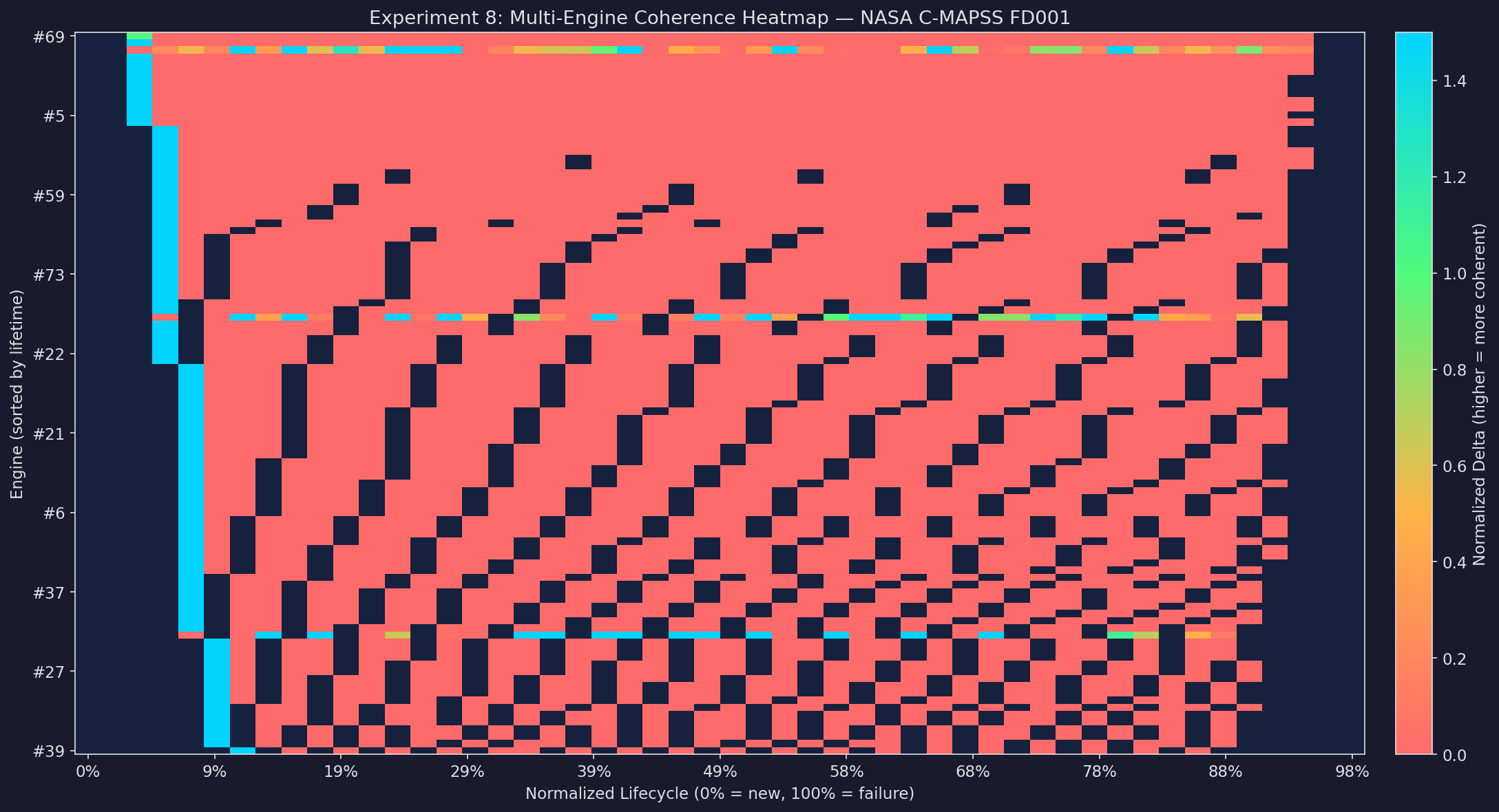
Multi-Engine Coherence Heatmap

100 engines sorted by lifetime. X-axis: normalized lifecycle (0% = new, 100% = failure). Color: coherence level (blue = coherent, red = degraded).

A clear universal pattern: coherence degrades progressively across the lifecycle. The transition from high to low coherence is visible across all engines, confirming that Δ captures a genuine physical degradation signal rather than noise. Universal Pattern

Notable Engines

Largest Δ advantage (top 5)

Engine	Lifetime	Δ Lead	Var Lead	Advantage
#92	341	320	0	+320
#96	336	320	0	+320
#67	313	292	15	+277
#86	278	257	0	+257
#95	283	262	16	+246

Smallest Δ advantage (bottom 5)

Engine	Lifetime	Δ Lead	Var Lead	Advantage
#29	163	142	115	+27
#27	156	135	109	+26
#36	158	137	111	+26
#65	153	132	106	+26
#77	154	133	107	+26

All Engines

Show all 100 engines

Engine	Lifetime	Δ Lead	Var Lead	Advantage
#1	192	171	113	+58
#2	287	266	104	+162
#3	179	158	113	+45
#4	189	168	21	+147
#5	269	248	155	+93
#6	188	167	120	+47
#7	259	238	142	+96
#8	150	129	0	+129
#9	201	180	145	+35
#10	222	201	72	+129
#11	240	219	76	+143
#12	170	149	100	+49
#13	163	147	75	+72
#14	180	159	38	+121
#15	207	186	150	+36
#16	209	188	112	+76
#17	276	255	110	+145
#18	195	174	105	+69
#19	158	137	91	+46
#20	234	213	22	+191
#21	195	174	55	+119
#22	202	181	131	+50
#23	168	147	44	+103
#24	147	126	60	+66
#25	230	209	0	+209
#26	199	178	144	+34
#27	156	135	109	+26
#28	165	144	71	+73
#29	163	142	115	+27
#30	194	173	140	+33
#31	234	213	47	+166
#32	191	170	37	+133
#33	200	179	64	+115
#34	195	174	0	+174
#35	181	160	129	+31
#36	158	137	111	+26
#37	170	149	75	+74
#38	194	173	45	+128
#39	128	107	76	+31
#40	188	167	20	+147
#41	216	195	157	+38
#42	196	175	136	+39
#43	207	186	150	+36
#44	192	171	138	+33
#45	158	137	51	+86
#46	256	235	39	+196
#47	214	193	26	+167
#48	231	210	89	+121
#49	215	194	36	+158
#50	198	177	143	+34
#51	213	192	30	+162
#52	213	192	50	+142
#53	195	174	90	+84
#54	257	236	95	+141
#55	193	172	139	+33
#56	275	254	104	+150
#57	137	116	25	+91
#58	147	126	95	+31
#59	231	210	109	+101
#60	172	151	37	+114
#61	185	164	77	+87
#62	180	159	0	+159
#63	174	153	14	+139
#64	283	262	51	+211
#65	153	132	106	+26
#66	202	181	111	+70
#67	313	292	15	+277
#68	199	178	24	+154
#69	362	341	99	+242
#70	137	116	50	+66
#71	208	192	26	+166
#72	213	192	65	+127
#73	213	192	85	+107
#74	166	145	92	+53
#75	229	208	168	+40
#76	210	189	152	+37
#77	154	133	107	+26
#78	231	210	29	+181
#79	199	178	109	+69
#80	185	164	17	+147
#81	240	219	111	+108
#82	214	193	36	+157
#83	293	272	54	+218
#84	267	246	193	+53
#85	188	167	115	+52
#86	278	257	0	+257
#87	178	157	77	+80
#88	213	192	35	+157
#89	217	196	43	+153
#90	154	133	57	+76
#91	135	114	23	+91
#92	341	320	0	+320
#93	155	134	68	+66
#94	258	237	56	+181
#95	283	262	16	+246
#96	336	320	0	+320
#97	202	181	101	+80
#98	156	135	69	+66
#99	185	164	22	+142
#100	200	179	124	+55

Dataset

NASA C-MAPSS FD001 — Commercial Modular Aero-Propulsion System Simulation. 100 turbofan engines run to failure under a single operating condition (sea level). 21 sensor channels + 3 operational settings per cycle. Mean lifetime: 206 cycles. Source: NASA Prognostics Center of Excellence.

Configuration — Baseline: first 20% of cycles. Window: 30 cycles, step 5. Δ threshold: 0.3. Sensors: s2, s3, s4, s7, s11, s12 (highest degradation signal).

Python NumPy SciPy NASA C-MAPSS FD001 100 Engines

Navigation

← Back to all experiments

Engine	Lifetime	Δ Lead	Var Lead	Advantage
#29	163	142	115	+27
#27	156	135	109	+26
#36	158	137	111	+26
#65	153	132	106	+26
#77	154	133	107	+26

Engine	Lifetime	Δ Lead	Var Lead	Advantage
#29	163	142	115	+27
#27	156	135	109	+26
#36	158	137	111	+26
#65	153	132	106	+26
#77	154	133	107	+26

Δ.72 on NASA C-MAPSS Turbofan