Δ.72 Mathematical Foundations

Implemented Modules

Tier 1 — Core Validation

RQA — Recurrence Quantification Analysis

Nonlinear Dynamics Validation of Pattern Retention

DET (determinism) and LAM (laminarity) track the system's dynamical structure through recurrence plots. Validates that Δ's P component captures genuine dynamical degradation, not just linear decorrelation.

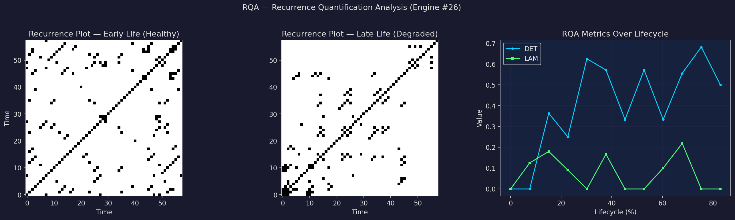
Multi-engine validation

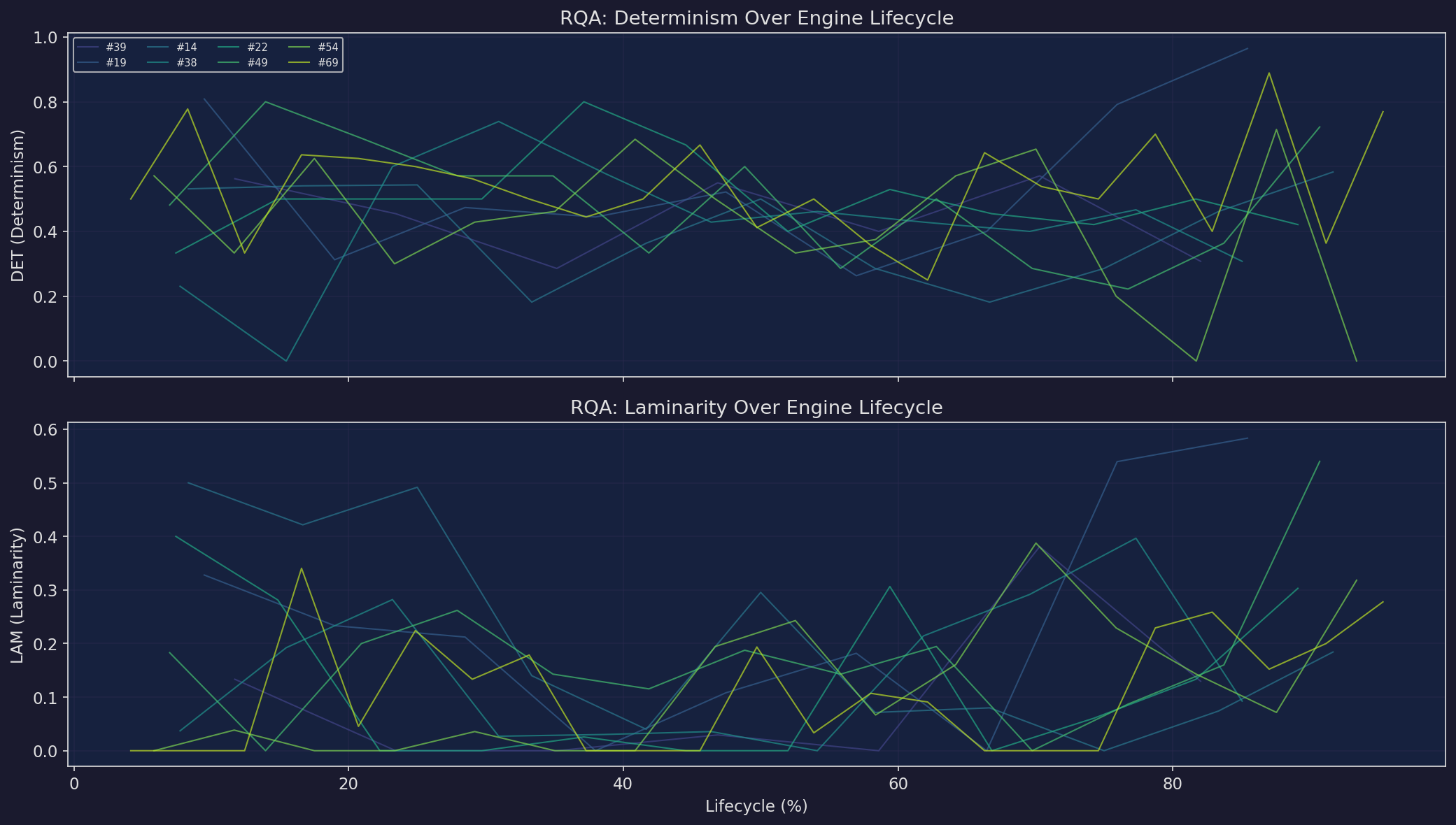
DET and LAM show characteristic evolution over engine lifecycle, confirming that coherence loss maps to genuine nonlinear dynamical degradation. Nonlinear Validated

Wavelet Coherence — Multi-Scale Decomposition

Scale-Resolved Coherence Spectrum

Morlet wavelet transform decomposes coherence into fast, medium, and slow timescales. Reveals whether degradation appears first at fast or slow scales.

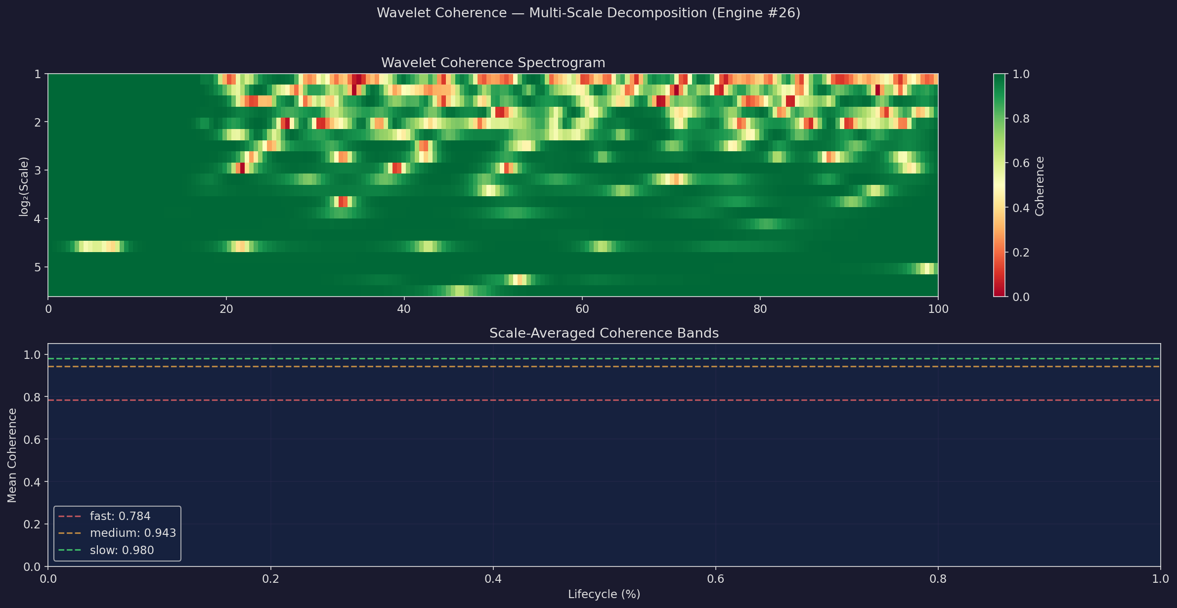
Multi-engine validation

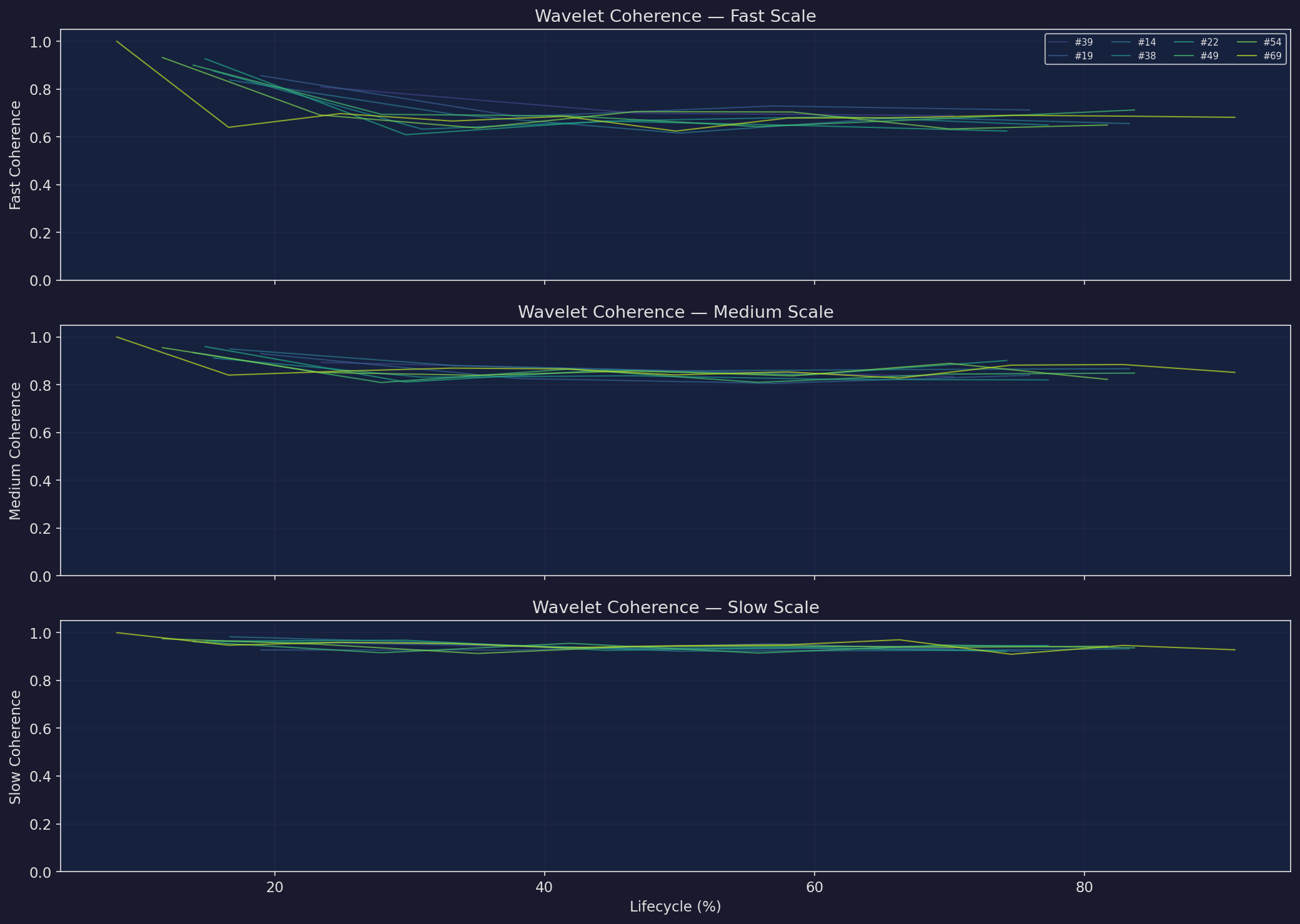
Coherence loss at different timescales follows distinct patterns across the engine lifecycle, validating the multi-scale nature of degradation. Multi-Scale

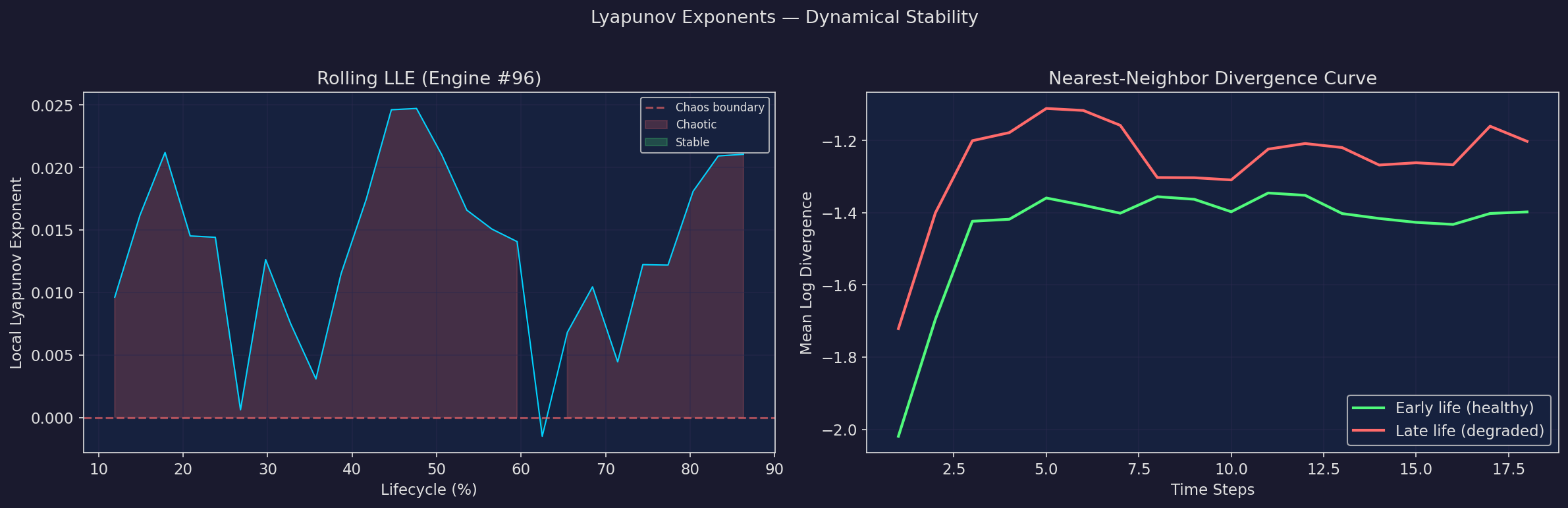
Lyapunov Exponents — Dynamical Stability

Rolling Local Lyapunov Exponent

The largest Lyapunov exponent (LLE) measures sensitivity to initial conditions. Positive LLE = chaotic, negative = stable. Rolling LLE tracks the system's approach to chaos over the degradation trajectory.

Multi-engine validation

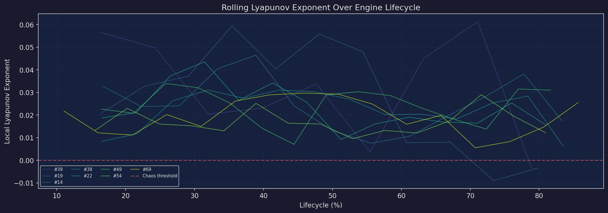
Engine	Regime
#39	chaotic
#19	edge
#14	edge
#38	edge
#22	edge
#49	edge
#54	edge
#69	edge

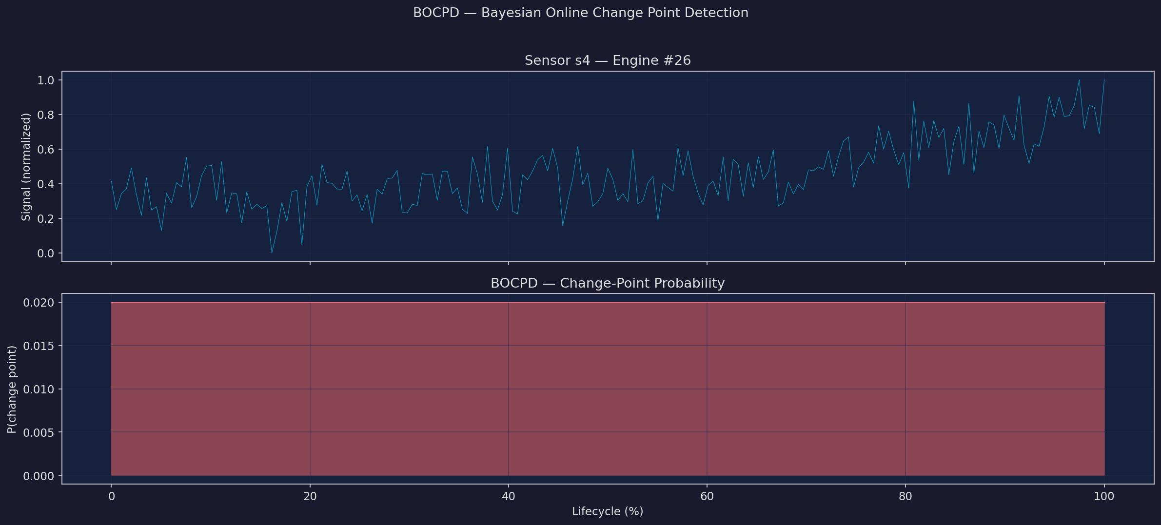
BOCPD — Bayesian Online Change Point Detection

Benchmark Competitor: Change Points vs Δ Alerts

Direct comparison: when does BOCPD detect a change point vs when does Δ drop below threshold? Green vertical lines = BOCPD change points.

Multi-engine validation

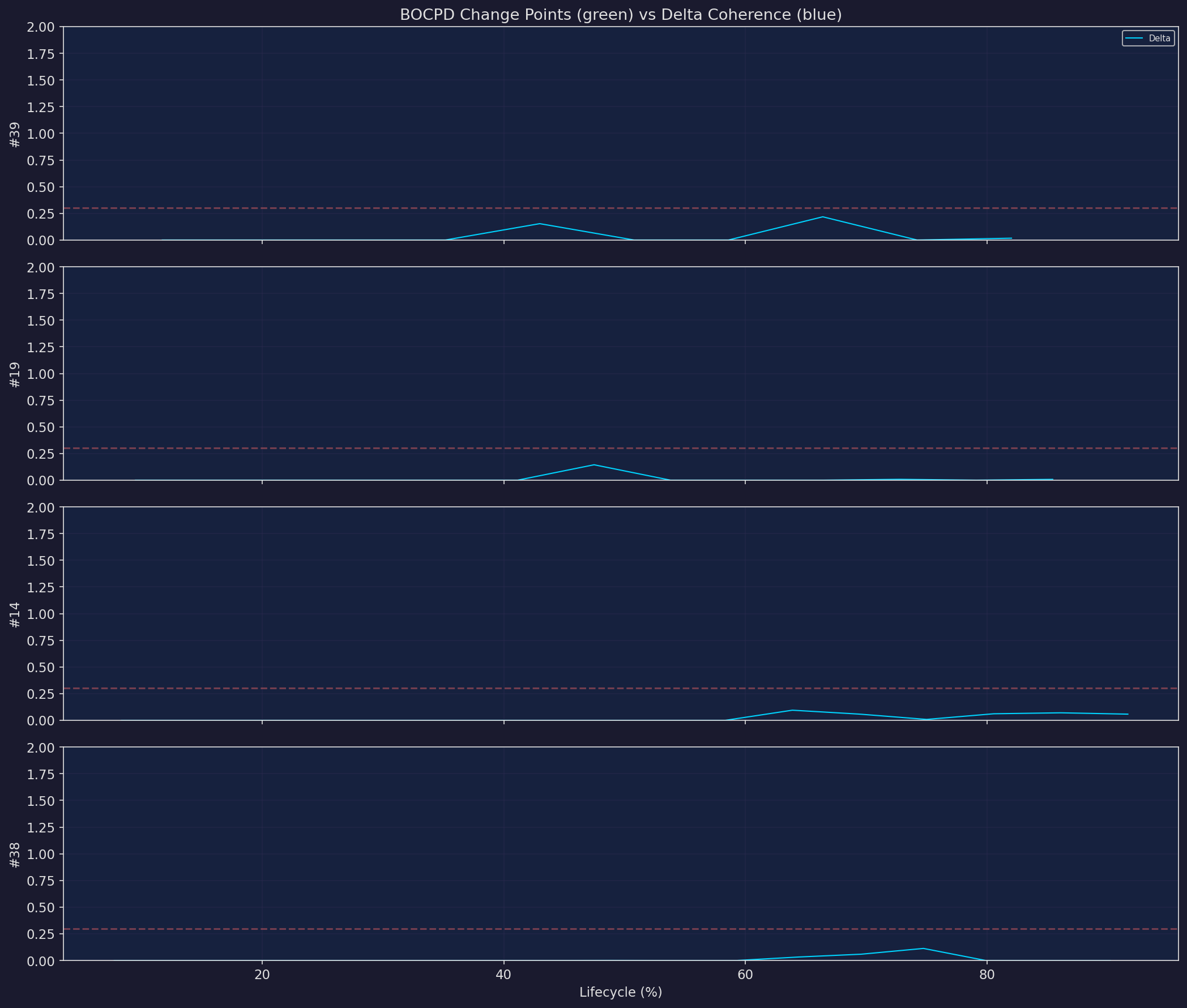
Engine	BOCPD Change Points
#39	0
#19	0
#14	0
#38	0
#22	0
#49	0
#54	0
#69	0

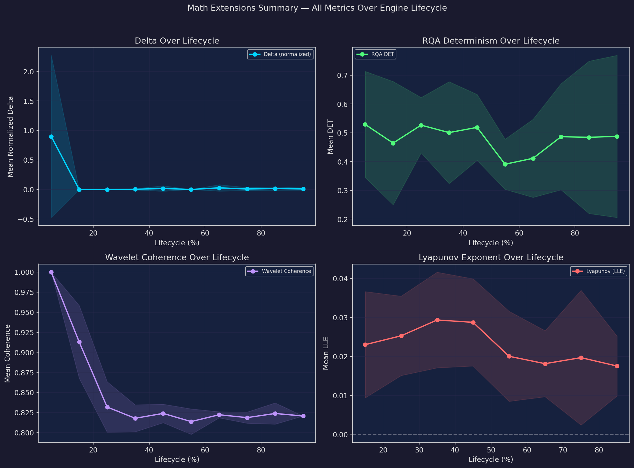
Combined Summary

All Metrics Over Engine Lifecycle

Lifecycle-binned averages of Δ, RQA Determinism, Wavelet Coherence, and Lyapunov exponent across all 8 sample engines.

Tier 2 — Advanced Extensions

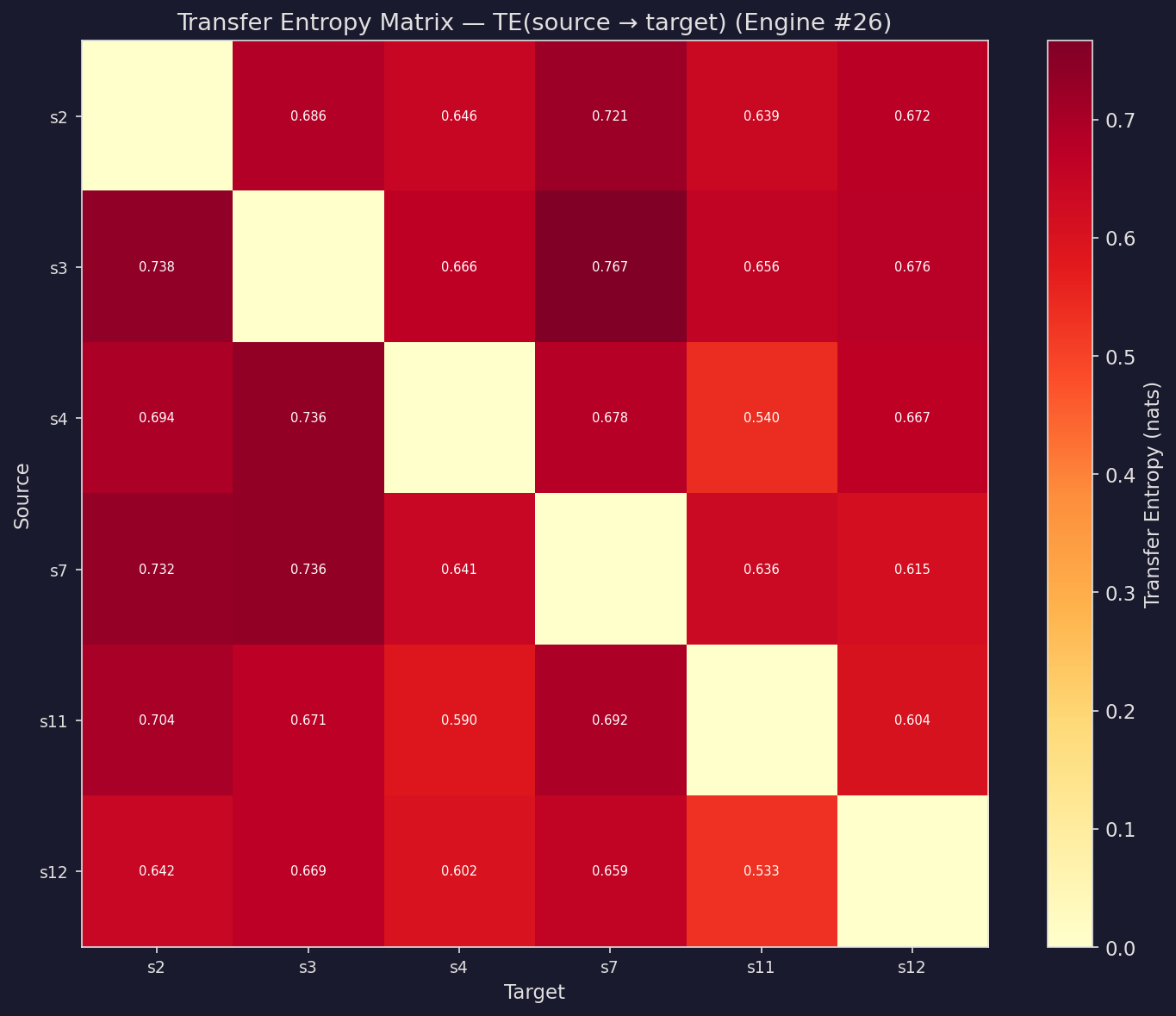
Transfer Entropy — Directed Information Flow

Causal Structure Between Sensors

TE(X→Y) measures how much X's past reduces uncertainty about Y's future. The matrix reveals which sensors drive degradation in others.

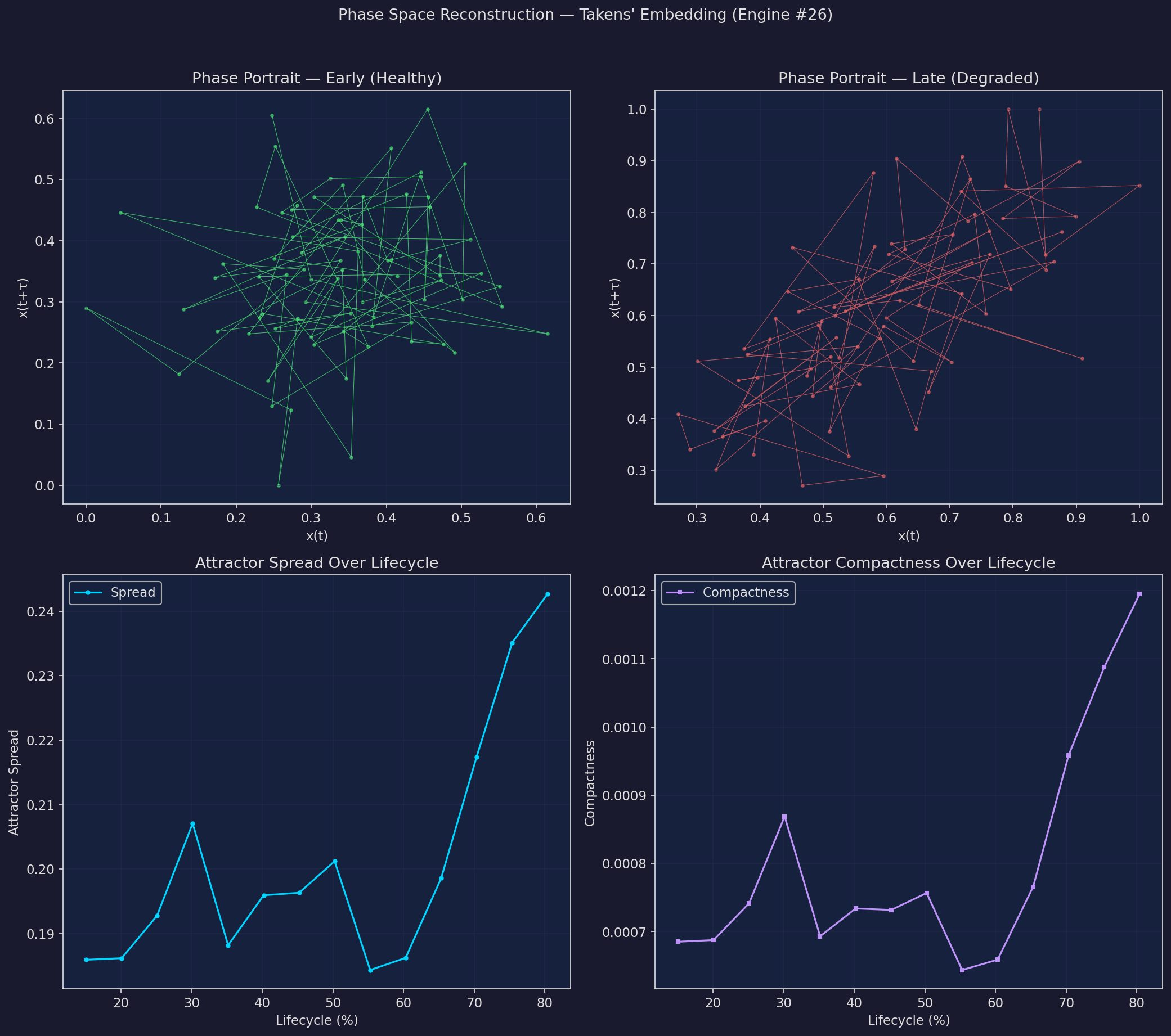
Phase Space Reconstruction — Takens' Embedding

Attractor Geometry: Healthy vs Degraded

Time-delay embedding reconstructs the system's attractor. Healthy = compact orbit. Degraded = smeared, expanding attractor.

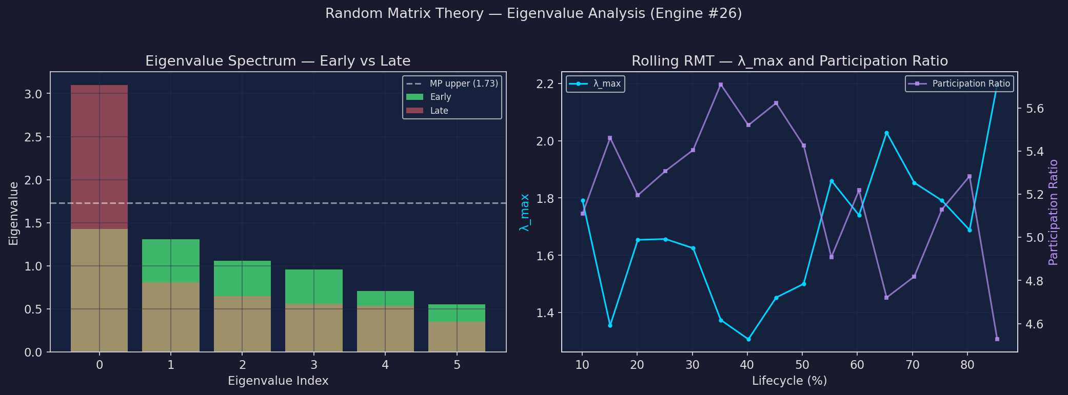
Random Matrix Theory — Eigenvalue Analysis

Marchenko-Pastur Bounds + Rolling λ_max

Multi-sensor correlation matrix eigenvalues. Signal eigenvalues exceed the Marchenko-Pastur noise bound. Inspired by Charles Martin's WeightWatcher.

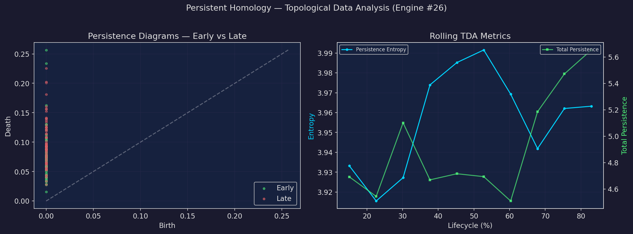
Persistent Homology — Topological Data Analysis

Persistence Diagrams + Rolling Entropy

Tracks the "shape" of data as it evolves. Points far from the diagonal represent stable topological features.

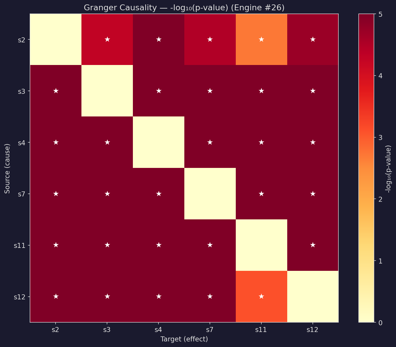
Granger Causality — Statistical Causation

Pairwise Causal Network Between Sensors

F-test for whether one sensor's past helps predict another. Stars (☆) mark statistically significant causal links (p<0.05).

Tier 3 — Research Frontier

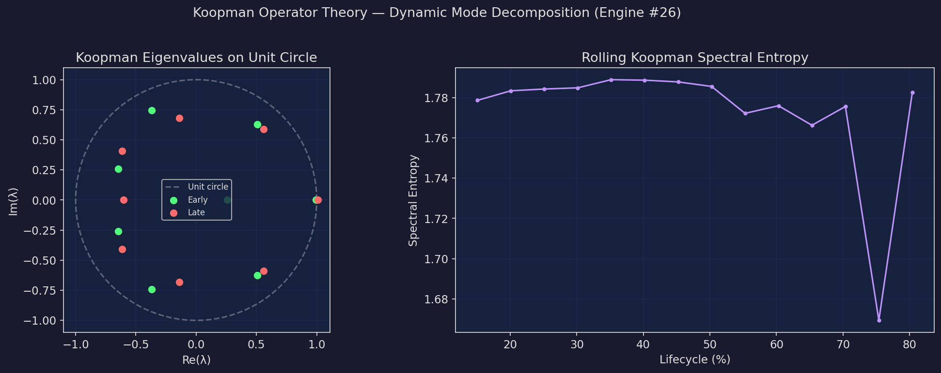
Koopman Operator Theory — Dynamic Mode Decomposition

Eigenvalues on the Unit Circle + Spectral Entropy

DMD approximates the Koopman operator. Eigenvalues inside the unit circle = decaying modes (stable). Outside = growing modes (unstable).

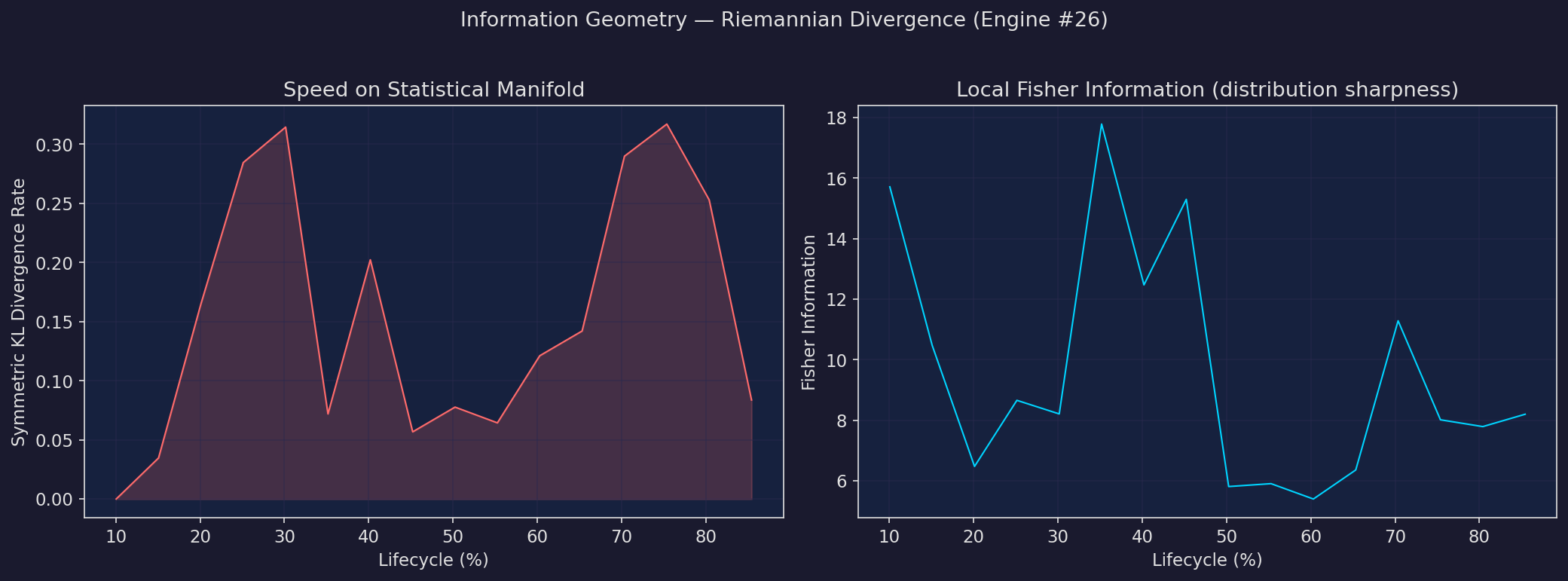
Information Geometry — Riemannian Divergence

Speed on the Statistical Manifold + Fisher Information

Measures how fast the signal's probability distribution is changing. High divergence rate = rapid state transition = approaching failure.

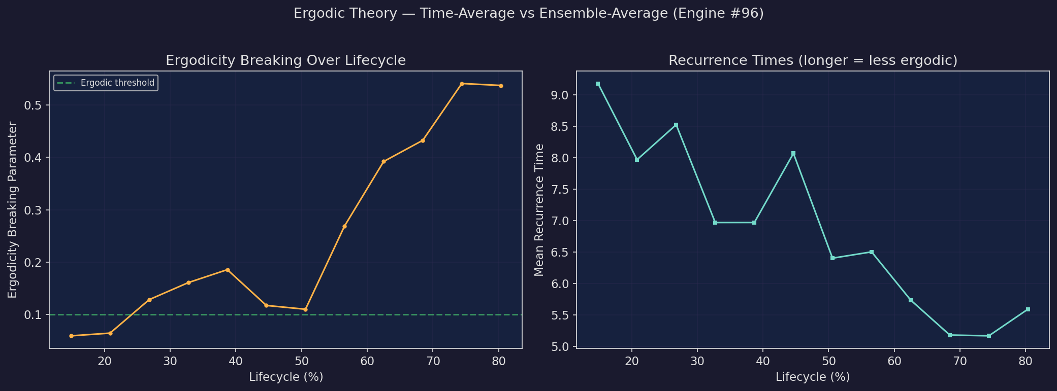
Ergodic Theory — Time vs Ensemble Averages

Ergodicity Breaking + Recurrence Times

A coherent system is ergodic (time averages = ensemble averages). Loss of ergodicity signals a phase transition in the system's dynamics.

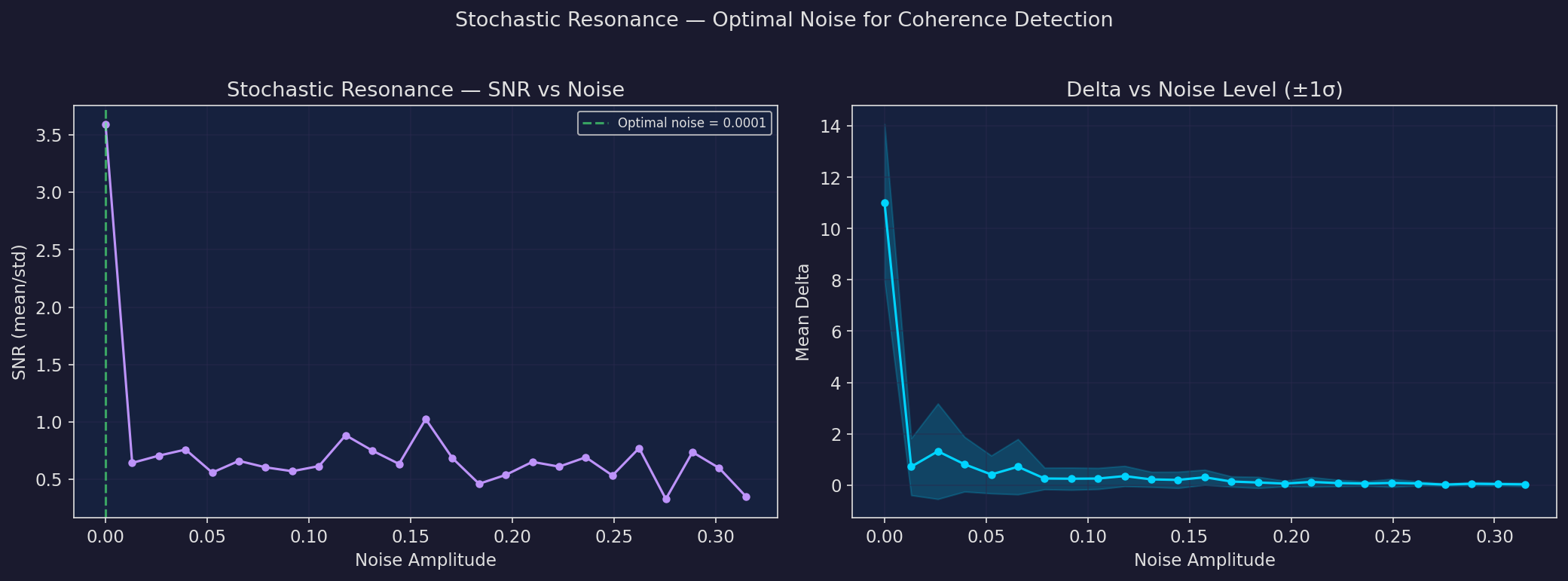
Stochastic Resonance — Optimal Noise

SR Curve: Signal-to-Noise Ratio vs Noise Level

Noise can enhance signal detection in nonlinear systems. The SR curve reveals the optimal noise level for coherence measurement — connecting to why the 0.72 threshold exists.

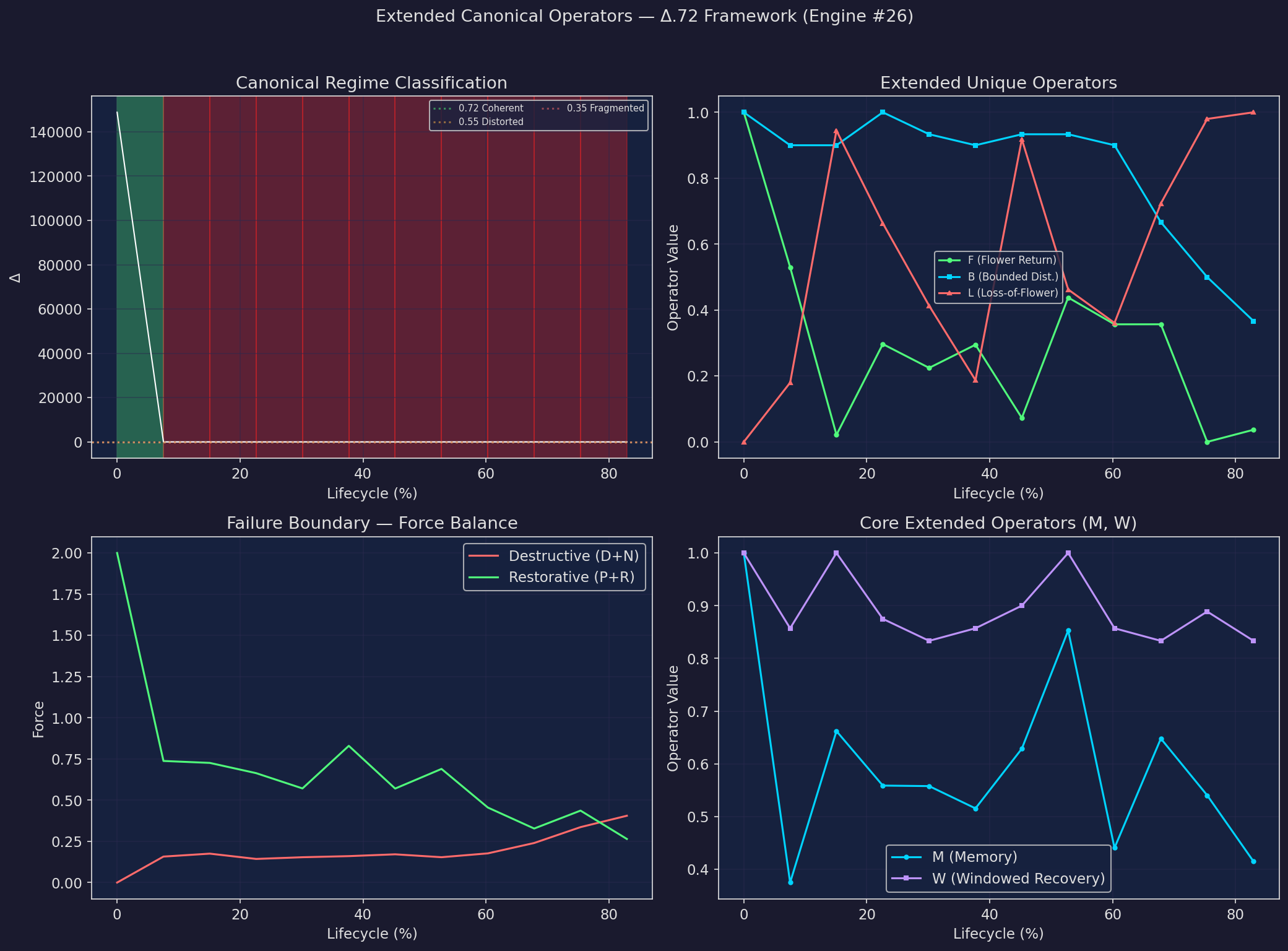
Extended Canonical Operators — Δ.72 Framework

Regime Classification + F/B/L Operators + Failure Boundary

The five extended operators from the canonical algorithm. Regime map shows the four phases (Coherent/Distorted/Fragmented/Collapse). Force balance tracks the failure boundary condition.

Module Reference

All modules at src/delta72/ — pure numpy implementations, no external dependencies. Runtime: 1.7s for full validation suite.

Related

Δ.72 Canonical Framework — Full equation reference, dimensional analysis, regime boundaries, extended operators.

Coherence Engine — Live coherence scoring platform.